As a showcase for Cloud&Heat’s upcoming GPU cloud, this blog post summarizes the results of a hackathon organized by the IT team at Cloud&Heat. We set up and ran a Deep Learning application on four Nvidia Tesla P100 GPUs which we have in our lab for testing purposes.
Introduction
Deep Learning is one branch of the current Machine Learning buzz that has a multitude of diverse applications as well as a hunger for computational resources. It is used for image and speech recognition, translation or autonomous driving, just to name a few. In terms of hardware, GPUs remain the workhorse of Deep Learning, since both training and inference make use of matrix operations which can be accelerated on these devices. Despite Google’s TPU cloud, GPUs have a far greater application domain in other computationally demanding applications.
The application that we will use here is termed Neural Style Transfer.

It uses deep neural networks to combine the content information of one image (left) with the artistic style of another (artwork in the middle) in order to make it look as if it was painted by the same artist1.
The idea to do this with deep learning was kicked off in 2015 by a paper called A Neural Algorithm of Artistic Style by Gatys et al.
One basic ingredient is the usage of pre-trained deep convolutional neural networks such as the VGG19 network, which was trained for the ImageNet Large Scale Visual Recognition Challenge (ILSVRC) to categorize images into 1000 different classes. Since the trained networks have developed an abstract representation of objects as well as their visual representation, one can use that to interrogate the network when feeding it an image. Gatys et al. showed how to extract the essential content information (e.g. the features of a face), as well the artistic style (e.g. brush strokes). Now one can use an optimization algorithm starting from a white noise image (or the content image) with the objective that the final image shall have both the desired content and style.
This optimization-based approach has the advantage that it can combine any given content with any style image. A faster approach was given by Johnson et al. and later refined by Ulyanov et al. where they train a second “transfer network” to solve the optimization in one forward pass. Once trained, the method is very fast, in fact one can even transfer videos in real time. However, the style image and all free parameters of the transfer are fixed. Also, to train the transfer network, one needs a large database of content images. Since we need a method to quickly load our GPUs, we go with Gatys’s method, were we only need one content and one style image.
There are many implementations of Gatys’ method such as this from Keras, this from Johnson or this from Athalye. We chose the latter TensorFlow implementation since it has a couple of parameters to play with. We use this as a nice showcase to illustrate a problem that everybody has to solve: parameter tuning. There are at least six parameters in our chosen implementation that influence the generated image. The ratio in which to weight style and content is just one example (hint: 50:50 is not it). With the computational power we have available, we can run many style transfer calculations in an orderly fashion to scan for the best parameters. Note that also the fast method of Johnson from above has to do this first in order to define the objective function for training the transfer network.
There are also newer advanced methods for Style Transfer based on Generative Adversarial Networks (CycleGANs) with impressive results which we won’t use here, however.
Before we go on, we’ll tell you about the hardware and software that we have used. If that is not your cup of tea then skip ahead — we also have Jupyter notebooks down there!
Hardware and Operating System
Our test machine is composed of a Supermicro chassis, a Supermicro X10DRG-OT+-CPU motherboard, 24 GB RAM and 24 CPU cores in a dual socket Intel Xeon E5-2650 setup. The case houses 4 Nvidia Tesla P100 GPUs (Pascal architecture), connected via PCIe (no NVLink). These cards are datacenter-grade devices, packing 16 GB of RAM per card and having 5, 11 and 21 Tflops peak performance in double (64bit), single (32bit) and half (16bit) precision mode, respectively.
We run Ubuntu 16.04 LTS on the bare metal host. In order to showcase the cloud usage scenario, we spin up a VM using 20 GB of RAM and 20 vCPUs, also running an Ubuntu 16.04 image. The machine resides in our lab and is not integrated into our OpenStack cloud, which is why we run it “by hand” using QEM in KVM mode driven by libvirt] and remote controlled by virt-manager. Each of the four P100s is attached as PCI device to the VM (GPU pass-through). We also pass all host CPU features through to the VM for maximal performance.
TensorFlow and CUDA
There are TensorFlow Docker images available, but we show here that it is easy to install TensorFlow along with all dependencies. After all, installing stuff is what our DevOps engineers do all day!
What we need to install for TensorFlow to work with the GPUs is
- the Nvidia device driver
- the CUDA Toolkit with GPU-enabled numerical libraries and more
- cuDNN: Nvidia library with GPU-accelerated primitives for deep neural nets
Since TensorFlow is C++ wrapped with Python, we can install it using pip. The current CUDA version is 10.0, but TensorFlow supports 9.0 at the time of writing. Ubuntu 16.04 ships CUDA 7 (nvidia-cuda-dev package), so we will install directly from Nvidia.
$ wget http://developer.download.nvidia.com/compute/cuda/repos/ubuntu1604/x86_64/cuda-repo-ubuntu1604_9.0.176-1_amd64.deb
$ sudo apt-key adv --fetch-keys http://developer.download.nvidia.com/compute/cuda/repos/ubuntu1604/x86_64/7fa2af80.pub
$ sudo dpkg -i cuda-repo-ubuntu1604_9.0.176-1_amd64.deb
$ sudo apt-get update
$ sudo apt-get --no-install-recommends install cuda-9-0
Installing CUDA packages should also pull a recent driver package, e.g. nvidia-410.
TensorFlow from pip is linked against cuDNN. You can get this from Nvidia after registration, which lets you download a Debian package.
$ sudo dpkg -i libcudnn7_7.2.1.38-1+cuda9.0_amd64.debNow we can install TensorFlow. We need to make sure to use the GPU-enabled version tensorflow-gpu:
$ sudo apt-get --no-install-recommends install python3-pip python3-wheel python3-setuptools
$ pip3 install tensorflow-gpu scipy matplotlib Pillow pandas psweep
While we were at it, we installed a couple of dependencies for the Style Transfer code (see below), namely scipy,matplotlib and the Pillow implementation of the Python Imaging Library (PIL). We also install psweep to help run and evaluate the parameter study.
That’s it!
Neural Style implementation
We forked the TensorFlow implementation of the Style Transfer algorithm described above and adapted it to our needs (basically convergence monitoring). The installation is straight forward. We just pull the repo and download trained weights of the VGG19 network:
$ git clone https://github.com/elcorto/neural-style
$ cd neural-style
$ wget http://www.vlfeat.org/matconvnet/models/beta16/imagenet-vgg-verydeep-19.mat
The executable which we use is neural-style/neural_style.py.
The algorithm uses the Adam optimizer, and the objective function to be optimized has three parts: the style_loss measures how well the output image reproduces the style of the style image, the content_loss does the same for content. The third component is the tv_loss (total variation regularization loss) which measures how smooth the image looks. The total loss is a weighted sum: total_loss = tv_weight * tv_loss + content_weight * content_loss + style_weight * style_loss.
Parameter tuning results
Our Style Transfer algorithm has many options, of which the following have been kept constant:
width = 512: Output image width. The height is determined from the content image’s aspect ratio. Our content and output images have 512×532 pixel.iterations= 1000: Most runs are converged after ~500 iterations, but with 1000, we are on the safe side.initial= None: We use a random white noise image for each run and not the content image. Because of this, no run, even with unchanged parameters, will have the exact same result.pooling= max: We use the default max pooling (instead of average pooling).
We scan the following parameters of the Style Transfer algorithm in order to find the visually most appealing results:
- learning_rate: The learning rate is the step size of the optimizer. To small values result in slow convergence, while too large values cause large jumps in the objective function value (
total_loss) and unstable convergence. style_scales: scale factor of the style image w.r.t. the output image, can select smaller or larger features in the style imagestyle_weight: weight forstyle_loss, we keepcontent_weight= 1, so this is the ratio of style/content mixing in the final imagetv_weight: weight oftv_losscontent_weight_blend: mixing factor for combining two content layersconv4_2*content_weight_blend+conv5_2* (1 –content_weight_blend), has an effect similar tostyle_weight- >code>style_layer_weight_exp: style layer weight exponential increase, similar to
content_weight_blendbut for style layers,weight(layer<n+1>)=weight_exp*weight(layer<n>), low values favor fine features of the style image over coarse ones
As you can see, the parameters above do all influence the final image, but even if one knows the general effect of a parameter, one needs a lot of test runs to find a good parameter combination. Side note: This is in itself an optimization problem. If we had a good metric to calculate how “visually appealing” an image is, we could let an algorithm find the best setting. But we don’t have that, so we need manual visual inspection.
Let’s say we like to test 10 values for each of the six parameter. Doing a brute force sampling would result in one million calculations. With one minute per run, this would take 10^6/60/24/365 = 1.9 years on one GPU. A bit long.
Assuming that the parameter effects are largely independent, we can take a much simpler approach: We use a set of default parameter values and vary each parameter independently. With 10 values per parameter, we would need only 60 runs, e.g. one hour on one GPU. We have four GPUs and can thus start four independent runs in parallel, which drops the calculation time to 15 min.
Here are the default parameters that we used.
Constant for all runs:
| width | 512 |
| iterations | 1000 |
| initial | None |
| pooling | ‘max’ |
| content_weight | 1 |
Defaults of parameters which have been varied:
| learning_rate | 10 |
| style_scales | 1 |
| content_weight_blend | 0.2 |
| style_weight | 10 |
| tv_weight | 100 |
| style_layer_weight_exp | 1 |
We performed 252 runs in total, sampling all parameters with 13 to 75 values. This takes about an hour on four GPUs. Here are some example results showing just 5 values (columns) per parameter (rows).

We have put the parameter study database, a compressed version of all result images and all scripts which we used to run the parameter study and evaluate the data in a GitHub repo, along with a Jupyter notebook where you can explore the full dataset. To do this interactively in your browser, start the Jupyter notebook here. This will use Binder to start a Docker container, checkout the repo, install all dependencies, start a Jupyter kernel and server and show you the notebook. If an already built Docker image of the repo is found, then this makes things start quicker. Once the notebook is loaded, click “Run”. It will take some seconds to render and download all six visualizations, which will look like this:

Then use the sliders to change the parameter values and observe how they affect the image.
You can also run that locally:
$ mkvirtualenv styletransfer -p /usr/bin/python3
$ git clone https://github.com/CloudAndHeat/style_transfer_parameter_sweep
$ cd style_transfer_parameter_sweep
$ pip3 install -r requirements.txt
$ pip3 install notebook
$ jupyter notebook interactive.ipynb
Performance
We ran preliminary CPU-only tests on our VM (20 vCPUs) for 1000 iterations of optimization, using the same image (512×532 pixel) as in all GPU runs. Note that TensorFlow uses all available cores by default, so any fair comparison must take the number of cores and the CPU type into account. We also ran a single-CPU test by forcing TensorFlow onto one CPU (using taskset -c 0 for CPU #0).
| 1 vCPU | ~4 hours 30 min (270 min) |
| 20 vCPU | 45 min |
| 20 vCPU + 1 GPU | 1 min |
The CPU-only speedup between 1 and 20 CPUs is only 270/45 = 6 instead of theoretically 20, which means that TensorFlow doesn’t scale well.
The run using one P100 finishes within 1 minute, so we have a factor 45 speedup! This is huge. Similar results have been obtained by a detailed Deep Learning benchmark performed by Microway, which covers the P100 and other Nvidia cards. Below we will show how to additionally leverage multiple GPUs with linear scaling.
Note that the image size has a large impact on the run time, since larger images result in larger matrices that must be processed.
Running on multiple GPUs
We use the psweep Python package to run the parameter study. It takes all parameter sets, runs the Style Transfer code for each and writes a database which we use to analyze the runs later. It can use multiprocessing to run each parameter set workload in parallel, which is what we do here. Since our use case is many independent calculations, multiprocessing is the ideal tool for parallelization, without using NVLink and multi-GPU TensorFlow. Also, this approach will scale linearly with the number of available GPUs.
We ran into two issues with TensorFlow. The first is that when running one instance of the Style Transfer code, TensorFlow will allocate memory on all four GPUs, even though it uses only one for computation. We can see this in the output of the nvidia-smi CLI tool.
+-----------------------------------------------------------------------------+
| NVIDIA-SMI 410.48                 Driver Version: 410.48                    |
|-------------------------------+----------------------+----------------------+
| GPU  Name        Persistence-M| Bus-Id        Disp.A | Volatile Uncorr. ECC |
| Fan  Temp  Perf  Pwr:Usage/Cap|         Memory-Usage | GPU-Util  Compute M. |
|===============================+======================+======================|
|   0  Tesla P100-PCIE...  Off  | 00000000:00:09.0 Off |                    0 |
| N/A   52C    P0   199W / 250W |  15639MiB / 16280MiB |     98%      Default |
+-------------------------------+----------------------+----------------------+
|   1  Tesla P100-PCIE...  Off  | 00000000:00:0A.0 Off |                    0 |
| N/A   37C    P0    35W / 250W |  15485MiB / 16280MiB |      0%      Default |
+-------------------------------+----------------------+----------------------+
|   2  Tesla P100-PCIE...  Off  | 00000000:00:0B.0 Off |                    0 |
| N/A   38C    P0    32W / 250W |  15485MiB / 16280MiB |      0%      Default |
+-------------------------------+----------------------+----------------------+
|   3  Tesla P100-PCIE...  Off  | 00000000:00:0C.0 Off |                    0 |
| N/A   45C    P0    34W / 250W |  15485MiB / 16280MiB |      0%      Default |
+-------------------------------+----------------------+----------------------+
+-----------------------------------------------------------------------------+
| Processes:                                                       GPU Memory |
|  GPU       PID   Type   Process name                             Usage      |
|=============================================================================|
|    0     26216      C   python3                                    15629MiB |
|    1     26216      C   python3                                    15475MiB |
|    2     26216      C   python3                                    15475MiB |
|    3     26216      C   python3                                    15475MiB |
+-----------------------------------------------------------------------------+
Note that the memory of all four GPUs is used, but only one has load (column GPU-Util). This is a known issue.
The second problem to solve is how to schedule tasks onto different GPUs when using multiprocessing. Our first approach was to use TensorFlow’s tf.device context manager in our fork of the Style Transfer code to select the GPU. This works as advertised. But we ran into the above issue again: We get OOM (out of memory) errors since, even if we schedule a second task correctly (one per GPU), memory is already allocated by the first task.
The solution to both problems is the environment variable CUDA_VISIBLE_DEVICES, which can be set to the ID of a GPU, for us 0,1,2 or 3. When running our code with this, we do not need tf.device at all, since the whole process will see only one GPU and allocate only on this. Inside the process, TensorFlow always sees one GPU only with ID 0, as in tf.device(‚/device:GPU:0‘), which is default.
The final piece to figure out is how to tell a process which GPU to use. There is a simple hack to do this. As it turns out, multiprocessing names the processes it starts something like ForkPoolWorker-1, ForkPoolWorker-2, etc. So we just have to parse the process name and turn that into the GPU ID. The code snippet below shows how we do this.
import multiprocessing
def worker(pset):
    """Run Style Transfer code for one parameter set (`pset`)."""
    ... here be code ...
def gpu_worker(pset):
    """Select GPU device based on multiprocessing process name."""
    name = multiprocessing.current_process().name
    # will set CUDA_VISIBLE_DEVICES={0,1,2,...}
    pset['gpu_device'] = int(name.replace('ForkPoolWorker-','')) - 1
    pset.update(worker(pset))
    return pset
if __name__ == '__main__':
    with multiprocessing.Pool(4) as pool:
        pool.map(gpu_worker, params)
This is an extremely simple trick to bind a multiprocessing process to a GPU. It is guaranteed to never oversubscribe a GPU since all four process will live as long as the main script runs, i.e. the binding is defined at startup and doesn’t change during the script’s run time.
Note that the pool.map() part above is not exactly how we do it, since we pass gpu_worker and params to psweep.run() which takes care of that. Here is the full script we used.
This is how it looks like in nvidia-smi
+-----------------------------------------------------------------------------+
| NVIDIA-SMI 410.48                 Driver Version: 410.48                    |
|-------------------------------+----------------------+----------------------+
| GPU  Name        Persistence-M| Bus-Id        Disp.A | Volatile Uncorr. ECC |
| Fan  Temp  Perf  Pwr:Usage/Cap|         Memory-Usage | GPU-Util  Compute M. |
|===============================+======================+======================|
|   0  Tesla P100-PCIE...  Off  | 00000000:00:09.0 Off |                    0 |
| N/A   63C    P0   182W / 250W |  15639MiB / 16280MiB |     98%      Default |
+-------------------------------+----------------------+----------------------+
|   1  Tesla P100-PCIE...  Off  | 00000000:00:0A.0 Off |                    0 |
| N/A   57C    P0   198W / 250W |  15639MiB / 16280MiB |     98%      Default |
+-------------------------------+----------------------+----------------------+
|   2  Tesla P100-PCIE...  Off  | 00000000:00:0B.0 Off |                    0 |
| N/A   65C    P0   199W / 250W |  15639MiB / 16280MiB |     98%      Default |
+-------------------------------+----------------------+----------------------+
|   3  Tesla P100-PCIE...  Off  | 00000000:00:0C.0 Off |                    0 |
| N/A   58C    P0   213W / 250W |  15639MiB / 16280MiB |     97%      Default |
+-------------------------------+----------------------+----------------------+
+-----------------------------------------------------------------------------+
| Processes:                                                       GPU Memory |
|  GPU       PID   Type   Process name                             Usage      |
|=============================================================================|
|    0     21788      C   python3                                    15629MiB |
|    1     21752      C   python3                                    15629MiB |
|    2     21821      C   python3                                    15629MiB |
|    3     21855      C   python3                                    15629MiB |
+-----------------------------------------------------------------------------+
Four GPUs at full load, this is what we like!
Conclusion
GPUs are without doubt powerful devices for numerical calculations with impressive speedups, when combined with GPU-enabled software. We showed how to set up a GPU machine and install TensorFlow and its dependencies. In the toy use case above, we demonstrated how to easily leverage multiple GPUs with plain Python multiprocessing built-in tools.
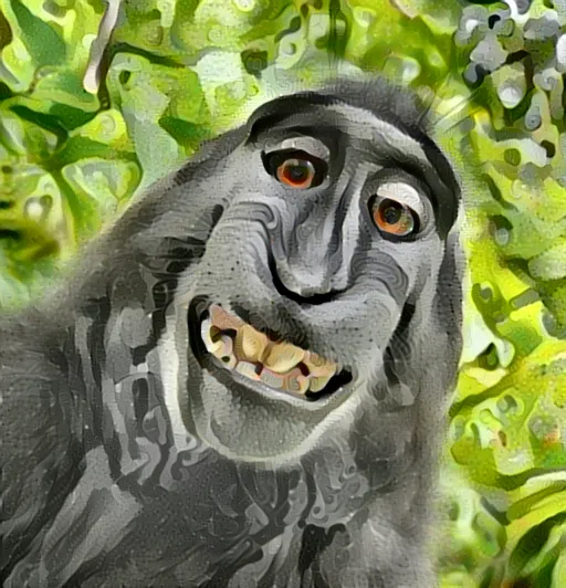
The „Candy“ style image is the same used by Johnson’s implementation, the „selfie“ content image is this from the Pexels database of public domain images.


